Neural Networks: How Artificial Brains Learn, Reason, and Power Modern AI

In my previous post, we took a deep dive into Large Language Models (LLMs)—breaking down how systems like ChatGPT and Claude take raw text, convert it into token IDs, and use probability distributions to predict the next word in a sequence.
At the very end of that article, a lot of developers asked me a fundamental question:
“You kept talking about weights, biases, layers, and embeddings… but what are those mathematical structures actually made of?”
The answer brings us to the absolute foundational building block of modern artificial intelligence: Neural Networks (specifically, Artificial Neural Networks or ANNs).
If LLMs are the sophisticated engines driving modern AI applications, Neural Networks are the raw physics of the engine itself. Without neural networks, there are no computer vision systems identifying objects in autonomous vehicles, no medical AI models diagnosing X-rays, no real-time speech translation, and no generative models.
In this guide, we are going to strip away the complex mathematical notation and academic jargon. We’ll explore how neural networks are built, how they actually “learn” from data, the different types of network architectures, and how you can understand them intuitively as a software developer.
Part 1: What is a Neural Network? (The Biological Analogy vs. The Mathematical Reality)
You’ll often hear people say that a neural network is an “artificial brain programmed inside a computer.”
While early AI pioneers in the 1950s (like Frank Rosenblatt, who built the first Perceptron) were inspired by biological brain cells, calling a neural network a human brain is a bit misleading.
Your biological brain contains roughly 86 billion neurons connected by trillions of synapses, communicating through complex biochemical and electrical pulses. An Artificial Neural Network, on the other hand, is a layered mathematical system designed to recognize complex patterns in numbers.
BIOLOGICAL NEURON                         ARTIFICIAL NEURON (PERCEPTRON)

     Dendrites (Inputs)                      Inputs (X1, X2, X3)
         \   /                                      \   |   /
        ── O ── Axon (Output)                        ── ⊙ ── Activation ──> Output (Y)
         /   \                                      /   |   \
     Dendrites (Inputs)                      Weights (W1, W2, W3) + Bias (b)
Think of a neural network as a massive, adjustable web of mathematical switches.
When you pass data into the network (like the raw pixels of an image or the financial metrics of a loan applicant), the numbers flow through thousands of tiny calculation points. Each point alters the data slightly until a final decision comes out the other side: “This image is a cat” or “This transaction is fraudulent.”
Part 2: The Anatomical Structure of a Neural Network
To understand how a neural network operates, we need to inspect its three core building blocks: Input Layers, Hidden Layers, and Output Layers.
+-----------------------------------------------------------------------+
|                    NEURAL NETWORK ARCHITECTURE                        |
+-----------------------------------------------------------------------+
|                                                                       |
|   INPUT LAYER           HIDDEN LAYERS             OUTPUT LAYER        |
|  (Raw Features)       (Feature Extraction)       (Final Prediction)   |
|                                                                       |
|     ( X1 ) ───────────── ( H1 ) ─────────────\                        |
|              \         /        \             \                       |
|               \       /          \             \                      |
|     ( X2 ) ────\──── ( H2 ) ──────\─────────── ( Y1 ) [Cat: 88%]      |
|                 \   /              \           /                      |
|                  \ /                \         /                       |
|     ( X3 ) ───── ( H3 ) ───────────── ( H4 ) ─ ( Y2 ) [Dog: 12%]      |
|                                                                       |
+-----------------------------------------------------------------------+
1. The Artificial Neuron (The Node)
The basic unit of a neural network is a single Node (or artificial neuron).
A node receives numerical inputs from the outside world (or from preceding nodes), calculates a weighted sum, adds a baseline adjustment (bias), passes the result through a mathematical filter (activation function), and fires the resulting output forward.
Every single artificial neuron performs one fundamental calculation:
$$Y = f\left(\sum (X_i \cdot W_i) + b\right)$$
Let’s unpack the four key ingredients of this formula:
A. Inputs ($X$)
The raw numerical data points fed into the neuron. If you are predicting house prices in Punjab, $X_1$ might be the square footage, $X_2$ might be the number of bedrooms, and $X_3$ might be the age of the property.
B. Weights ($W$)
Weights represent the importance or strength of each input connection.
- If the number of bedrooms ($X_2$) has a massive impact on the price, the network will assign a large weight ($W_2 = 8.5$) to that connection.
- If the color of the front door has zero impact, the network will assign a near-zero weight ($W_{door} = 0.01$).
Weights are the “memory” of a neural network. When an AI model is being trained, updating its knowledge simply means modifying these weight numbers!
C. Bias ($b$)
The bias is an extra numerical value added to the sum before passing it through the activation function.
Think of bias as a threshold modifier. Even if all your incoming input features ($X$) are zero, the bias allows the neuron to shift its decision line up or down. It ensures the neuron can still fire even when input values are low.
D. Activation Functions ($f$)
If a neural network only multiplied inputs by weights and added biases, it would just be a fancy linear regression model. It would only be capable of solving straight-line problems.
Real-world data is messy, complex, and non-linear. Activation functions introduce non-linearity into the network, enabling it to learn complex, curved decision boundaries.
                  COMMON ACTIVATION FUNCTIONS

     Sigmoid (0 to 1)             ReLU (Rectified Linear Unit)
        │    ┌──┐                      │        /
        │   ┌┘  └┐                     │       /
   ─────┼───┘────└─────           ─────┼──────/───────
        │                              │     /
│ │ / (If X > 0, output X)- ReLU (Rectified Linear Unit): The most widely used activation function in modern deep learning. If the input is negative, it outputs $0$. If the input is positive, it outputs the input directly ($X$). It is computationally fast and prevents network signals from saturating.
- Sigmoid: Maps any incoming number to a smooth value between $0$ and $1$. It’s often used in the final layer for binary classification problems (e.g., “Is this email Spam (1) or Not Spam (0)?”).
- Softmax: Used in multi-class output layers to transform raw score outputs into a clean probability distribution that sums up to $100\%$.
2. Layers of a Network
Neural networks organize their nodes into distinct operational tiers:
- Input Layer: Accepts the raw input features. If you feed a $28 \times 28$ pixel grayscale image into a network, your input layer will contain $784$ individual input nodes (one for each pixel brightness value).
- Hidden Layers: The magic happens here. A network can have anywhere from one hidden layer to hundreds of hidden layers (which is why it’s called Deep Learning).
- The first hidden layer might detect basic edges and lines in pixel data.
- The second hidden layer combines edges to recognize shapes (like circles or squares).
- Deeper hidden layers combine shapes to recognize complex concepts (like eyes, noses, or full human faces).
- Output Layer: The final node or group of nodes that delivers the network’s prediction (e.g., a classification label, a continuous price estimate, or token probabilities).
Part 3: How Neural Networks Learn (Training, Loss, & Backpropagation)
When a neural network is first created, its weights and biases are assigned completely random numbers. If you feed an image of a cat into an untrained network, it might guess with $99\%$ confidence that it’s a toaster.
How does a network turn from a random guesser into an accurate prediction system? Through a continuous feedback loop known as Training.
+-----------------------------------------------------------------------+
|                      THE NEURAL LEARNING LOOP                         |
+-----------------------------------------------------------------------+
|                                                                       |
|  1. FORWARD PASS      ─> Inputs travel forward to generate a prediction|
|            │                                                          |
|            ▼                                                          |
|  2. LOSS CALCULATION ─> Compare prediction against true target value  |
|            │             (Compute Error / Loss Score)                 |
|            ▼                                                          |
|  3. BACKPROPAGATION  ─> Calculate gradients (direction to fix weights)|
|            │                                                          |
|            ▼                                                          |
|  4. OPTIMIZATION     ─> Update weights using Gradient Descent         |
|            │                                                          |
|            └─────────── Repeat millions of times! ────────────────────┘
|                                                                       |
+-----------------------------------------------------------------------+
Step 1: The Forward Pass
During a forward pass, a training data sample (e.g., a handwritten digit image of the number 7) is fed into the input layer. The numbers flow through the hidden layers, node calculations are performed using the current weights and biases, and an output prediction is produced: “Prediction = 3”.
Step 2: Calculating Loss (The Error Function)
The network compares its prediction (3) against the actual ground-truth label (7). It uses a Loss Function (or Cost Function) to compute a single mathematical number representing how far off its guess was.
- Common Loss Function: Mean Squared Error (MSE) for regression problems, or Cross-Entropy Loss for classification tasks.
If the loss is high, the model performed poorly. The ultimate goal of training is to adjust the weights throughout the network until the Loss Score is as close to zero as possible.
Step 3: Backpropagation (The Engine of AI)
Invented in concept decades ago but popularized in the late 1980s by pioneers like Geoffrey Hinton, Backpropagation is the core algorithm behind modern AI.
Once the loss score is calculated at the output layer, backpropagation works backwards through the network—from the output layer, back through all the hidden layers, to the input layer.
Using calculus (specifically the Chain Rule), backpropagation calculates the Gradient for every single weight in the network.
The gradient tells us: “If I tweak this specific weight value slightly higher or lower, how much will the total error (loss) go down?”
                             Loss / Error
                                  │
                                 \│/  (Gradient Slope)
                                  ▼
                        \                  /
                         \                /
                          \              /
                           \   Current  /
                            \   Weight /
                             \   (O)  /  <── Goal: Roll down to minimum!
                              \______/
                           Global Minimum
Step 4: Optimization (Gradient Descent)
Once backpropagation calculates the gradients, an Optimizer (like Stochastic Gradient Descent (SGD) or Adam) updates the weights across the system.
$$\text{New Weight} = \text{Old Weight} – (\text{Learning Rate} \times \text{Gradient})$$
- The Learning Rate: A small multiplier (e.g., $0.001$) that controls how large of a step the optimizer takes when adjusting weights.
- If the learning rate is too high, the optimizer might overshoot the optimal point and cause the model to diverge.
- If the learning rate is too low, training will be painfully slow and might get stuck in a local minimum.
By repeating this Forward Pass $\rightarrow$ Loss Calculation $\rightarrow$ Backpropagation $\rightarrow$ Weight Update cycle over millions of training images or text passages, the network slowly shapes its weights until its predictions become incredibly accurate.
Part 4: Major Types of Neural Network Architectures
Just as software engineers choose different database types depending on the data model, AI researchers use different neural network architectures depending on the nature of the input features:
                          NEURAL NETWORK FAMILY TREE
                                      │
         ┌────────────────────────────┼────────────────────────────┐
         ▼                            ▼                            ▼
   DENSE / ANN                   CONVOLUTIONAL (CNN)           TRANSFORMERS
   (Feed-Forward)                (Computer Vision)             (Language & Sequence)
   - Tabular Data                - Image Classification        - LLMs (GPT, Claude)
   - Simple Predictions          - Object Detection            - Multi-modal Audio/Video
1. Feed-Forward Neural Networks (FNN / ANN)
The classic architecture where connections between nodes move in one single direction: forward from input to output, with no loops or cycles.
- Best Used For: Tabular structured data (like CSV spreadsheets, user churn predictions, or real estate pricing models).
2. Convolutional Neural Networks (CNNs)
Designed specifically for processing multi-dimensional spatial data like images and video streams.
Instead of connecting every single pixel to every node in a hidden layer (which would create billions of connections), a CNN slides small mathematical filters (called Kernels) across the image grid.
Input Image Grid (5x5)          Kernel Filter (3x3)           Feature Map
┌───┬───┬───┬───┬───┐              ┌───┬───┬───┐             ┌───┬───┬───┐
│ 1 │ 0 │ 1 │ 0 │ 0 │              │ 1 │ 0 │ 1 │             │ 4 │ 3 │ 1 │
├───┼───┼───┼───┼───┤   Sliding    ├───┼───┼───┤   ======>   ├───┼───┼───┤
│ 0 │ 1 │ 1 │ 1 │ 0 │  ───────>    │ 0 │ 1 │ 0 │             │ 2 │ 4 │ 2 │
├───┼───┼───┼───┼───┤  Convolution ├───┼───┼───┤             └───┴───┴───┘
│ 0 │ 0 │ 1 │ 0 │ 0 │              │ 1 │ 0 │ 1 │
└───┴───┴───┴───┴───┘ └───┴───┴───┘- How it works: As the filter slides over the image, it performs matrix multiplication to detect spatial patterns like vertical edges, horizontal lines, color gradients, and textures.
- Best Used For: Image classification, facial recognition, autonomous vehicle perception, and medical scan analysis.
3. Recurrent Neural Networks (RNNs) & LSTMs
Before Transformers dominated NLP, RNNs were the default choice for sequential data like speech, time-series data, and text.
- How it works: RNNs contain internal loop connections that allow outputs from previous steps to be fed back into the network alongside new inputs, giving the model a short-term memory of previous elements in a sequence.
4. Transformers (Attention-Based Networks)
The architecture behind modern LLMs, replacing sequential processing with parallel self-attention.
- How it works: Connects every element in an input sequence to every other element simultaneously, dynamically calculating context weights using self-attention heads (as covered in our LLM guide).
- Best Used For: Large Language Models, language translation, code generation, and multi-modal foundational AI systems.
Part 5: Building a Simple Neural Network in Code
To see how these concepts translate into real software, let’s build a basic Feed-Forward Neural Network in Python using PyTorch—the industry-standard framework used by AI engineers worldwide.
We will create a network that classifies incoming tabular feature data into one of two output categories.
import torch
import torch.nn as nn
import torch.optim as optim

# 1. Define the Neural Network Architecture
class SimpleNeuralNet(nn.Module):
    def __init__(self, input_dim, hidden_dim, output_dim):
        super(SimpleNeuralNet, self).__init__()

        # Layer 1: Input -> Hidden Layer (Linear transformation)
        self.fc1 = nn.Linear(input_dim, hidden_dim)

        # Non-linear Activation Function
        self.relu = nn.ReLU()

        # Layer 2: Hidden Layer -> Output Layer
        self.fc2 = nn.Linear(hidden_dim, output_dim)

        # Final Output Activation (Sigmoid for 0 to 1 probability)
        self.sigmoid = nn.Sigmoid()

    def forward(self, x):
        # Step 1: Pass inputs through 1st layer
        out = self.fc1(x)

        # Step 2: Apply ReLU activation
        out = self.relu(out)

        # Step 3: Pass through 2nd layer
        out = self.fc2(out)

        # Step 4: Apply Sigmoid activation to get final probability
        out = self.sigmoid(out)
        return out

# 2. Instantiate Network (4 Input features, 8 Hidden Nodes, 1 Binary Output)
model = SimpleNeuralNet(input_dim=4, hidden_dim=8, output_dim=1)

# 3. Define Loss Function and Optimizer
criterion = nn.BCELoss() # Binary Cross Entropy Loss
optimizer = optim.Adam(model.parameters(), lr=0.01) # Adam Optimizer

# 4. Dummy Input Data (Batch of 3 samples, 4 features each)
dummy_inputs = torch.tensor([
    [2.5, 1.2, 0.5, 3.1],
    [0.1, 4.2, 1.1, 0.8],
    [1.8, 0.4, 2.9, 1.5]
], dtype=torch.float32)

# Dummy Ground-Truth Target Labels (0 or 1)
dummy_targets = torch.tensor([[1.0], [0.0], [1.0]], dtype=torch.float32)

# 5. Execute Single Training Step (Forward + Backward Pass)
# Step A: Forward Pass
predictions = model(dummy_inputs)
loss = criterion(predictions, dummy_targets)

print(f"Initial Predictions:\n{predictions.detach().numpy()}")
print(f"Calculated Loss: {loss.item():.4f}")

# Step B: Backward Pass (Backpropagation)
optimizer.zero_grad() # Clear old gradients
loss.backward()       # Compute new gradients via Chain Rule
optimizer.step()      # Update network weights using calculated gradients

print("\nWeights successfully updated via Backpropagation!")
Part 6: Why Neural Networks Are Transforming Software Engineering
For decades, traditional software engineering followed a straightforward paradigm:
$$\text{Rules (Code)} + \text{Data} \longrightarrow \text{Outputs}$$
A human programmer had to manually write explicit if/else logic for every possible edge case. If you wanted a computer to detect fraudulent credit card transactions, you had to write thousands of hardcoded validation rules.
Neural networks flip this paradigm completely:
$$\text{Data} + \text{Desired Outputs} \longrightarrow \text{Rules (Learned Weights)}$$
Instead of writing rules manually, we feed millions of historical data examples (transactions paired with fraud labels) into a neural network. Through forward passes, loss evaluation, and backpropagation, the network discovers its own non-linear rules—finding subtle patterns across data features that no human software engineer could ever spot manually.
Conclusion
Neural networks aren’t magical biological entities; they are elegant mathematical systems combining linear algebra, matrix operations, activation functions, and calculus-based optimization.
Understanding these foundational concepts gives web and software developers a huge advantage. Whether you are consuming pre-trained model APIs, implementing local open-source models, tuning embeddings for a RAG search engine, or training your own custom ML pipelines, knowing how weights, loss functions, and backpropagation operate allows you to build faster, smarter, and more resilient software.
Have you started experimenting with frameworks like PyTorch, TensorFlow, or ONNX in your applications? Let’s discuss your implementation details or questions in the comments below!

25 year old AI & MERN Stack Developer based in Mohali, Punjab, India, with a strong interest in system design, Artificial Intelligence, Large Language Models (LLMs), and scalable software architecture. Passionate about building innovative, intelligent, and high-performance applications.